This week's lab focused on mapping damage from coastal flood events and the creation of impact analyses for buildings in low lying areas that would run the risk of inundation from storm surge in the event of extreme weather.
For the first step of this exercise, we were provided with storm indextiles containing two LiDAR files for the coastal town of Mantoloking, New Jersey in 2012. That year, hurricane Sandy struck and caused considerable coastal damage. One of the two LiDAR images provided was taken befoe the hurricane struck and the other six days after the event. We extracted a digital elevation model from the files and subtracted the pre-hurricane DEM from the post hurrricane DEM. The colors were switched to a value range of blue to red. Blue represented areas where the little to no elevation was lost and red highlighted areas where there had been a megative differential in elevation values. Red was chosen to display this loss as red is more pronounced on a blue background, allowing us to easily identify the areas most impacted by the storm. Below is a map made of our results.

Next we were given two DEMs of the coast if New Jersey. We isloated all of the pixels that represented an elevation of two meters as this height and all areas below would be considered to be vulnerable to storm surge. We reclassififed the raster, coverted it so a polygon, and then performed a clip with a polygon of Cape May to isolate the two meter and below areas that exist within Cape May. We found that 46.85% of Cape May is vulnerable to a two meter storm surge.
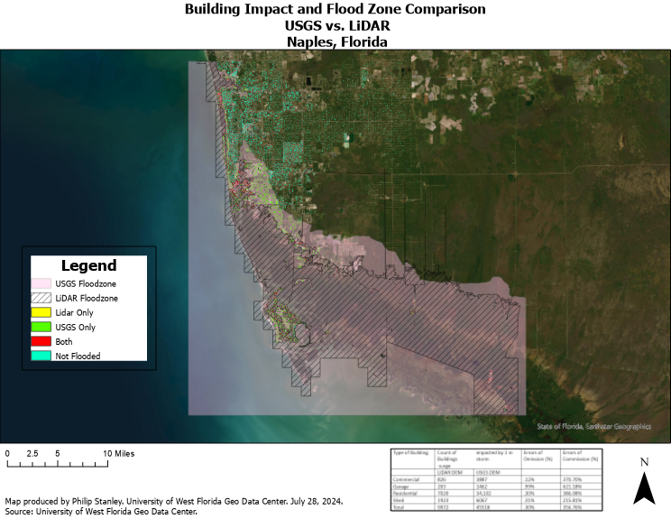
The final part of the lab had us taking two DEMs of Naple, Florida, one created by the USGS while the other was captured with LiDAR. We were tasked with creating a layer that represented all elevations below one meter. These would be areas considered vulnerable to storm surge abd thus described as floodplains.
This step was rather challenging as we had many values on the mainland portion of the image that had elevations below one meter, however, we were only intersted coastal geographies so we had to separate them. This involved using the Region Group tool which lumps together under distnct values all connecting values into seperate classes. We could then select these homogenos regions and convert them to polygons. This gave us the flood zones as recorded by LiDAR and the USGS.
We were then given a point feature class of all of the buildings in the area. We compared which DEM covered the buildings and used SQL queries to see which DEMs covred which buildings. The larger and less inaccurate USGS survey covered a tremendously greater area of buildings while the more accurate covered fewer. We then examined which buildings shared a floodzone and which resided exclusively in one and which were not in a flood plain. This information was then displayed in the map below. The error of omission was performed for the LiDAR to determine its missed houses and resulted in .30%. To test the accuracy of the larger USGS survey, the error of commission was found by quantifying the buildings that did not also lie in the LiDAR polygon. Due to the size of of the USGS survey, it was not accurate. The map iis below.
Comments
Post a Comment